Continuous problems
Contents
Simple, convex test-function
x=linspace(-4,4,200);
y=x;
[xx,yy]=meshgrid(x,y);
mesh(x,y,xx.^2+yy.^2);
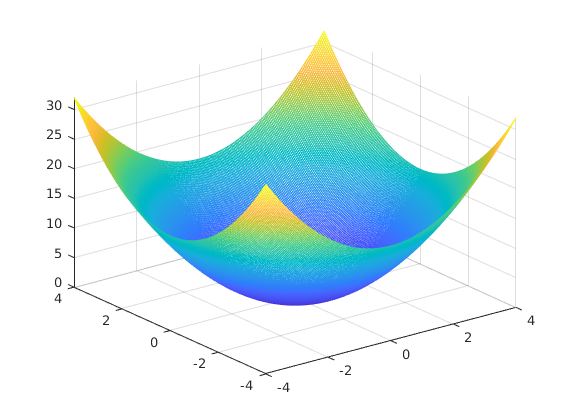
The global minimum is the origin, each algorithm can use at most 500 function evaluation.
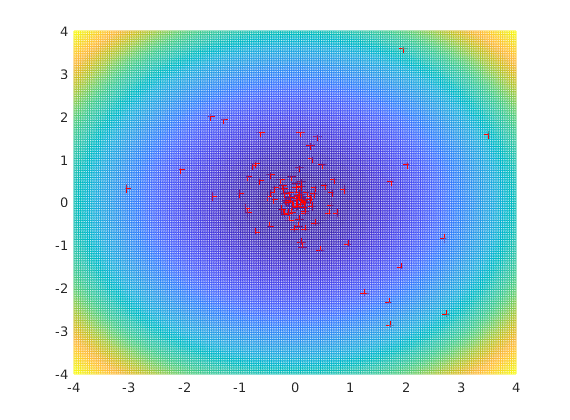
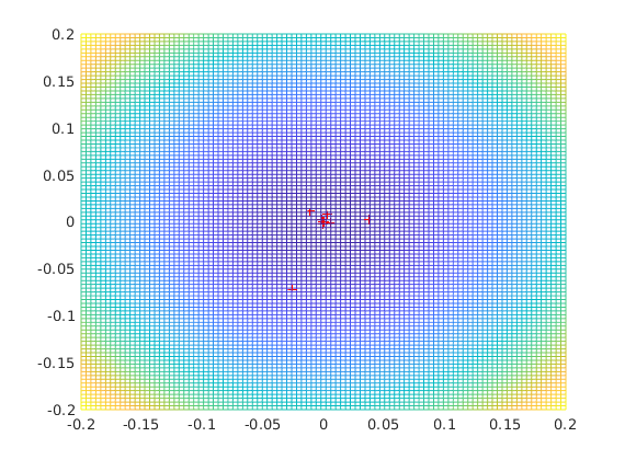
Simulated annealing
figure(2)
xMin=hutes_abra(1,1,5,2,0.2,100,@(x)x(1)^2+x(2)^2)
xMin =

    0.1470
    0.0608
Rechenberg's algorithm
figure(3)
rechenberg_abra(@(x) x(1)^2+x(2)^2,[1,1])
ans =

   -0.0024   -0.0123

Evolutionary strategy
figure(4)
esUc1_abra(@(x) x(1)^2+x(2)^2,2)
ans =

   1.0e-03 *

    0.3384   -0.1276    0.6521
Uncorrelated Evolutionary strategy
figure(5)
esUcn_abra(@(x) x(1)^2+x(2)^2,2)
ans =

    0.0003   -0.0004    0.0005    0.0016

Long valley problem
figure(6)
x=linspace(-4,4,200);
y=x;
[xx,yy]=meshgrid(x,y);
mesh(x,y,10000*xx.^2+yy.^2);

It takes time the learn the directions, but might worth the effort
esUc1(@(x) 10000*x(1)^2+x(2)^2,2)
ans =

   -0.0006   -0.0713    0.0043
esUcn(@(x) 10000*x(1)^2+x(2)^2,2)
ans =

    0.0033    0.2195    0.2027    3.0503
Recommended problem
Compare this algorithms to the gradient-method!