Interpolation
Contents
We have the following problem: there is an unknown background function, and at some point we measured the value of the function. Our goal is to determine the value of the function (based on the measurements) at some point which falls into the interval determined by the of the known points.
Linear interpolation
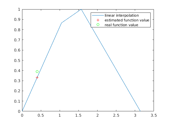
We simply draw segment between our data points, and estimate the function value by the high of the corresponding segment. For example:
Data points
x=[0 pi/3 pi/2, pi];
Measured data:
y=[0 sqrt(3)/2 1 0];
The point where we want to determine the function value:
point1=0.4;
Estimate based on linear interpolation
value1=interp1(x,y,point1)
value1 =

    0.3308
It's easy to calculate, but isn't accurate, and only uses the two neighboring points. In our example the background function was a sine function, which is a concave one on that interval, but the information about convexity is lost, if we use linear interpolation.
plot(x,y, point1,value1,'r+',point1,sin(point1),'go')
legend('linear interpolation', 'estimated function value', 'real function value')
Spline interpolation
Instead of segments a popular method uses 'smooth' (piecewise qubic polynomials) to interpolate data. The resulting interpolation function is continuous and differentiable. This method is called spline interpolation.
ert2=spline(x,y,point1)
ert2 =

    0.4189
t=linspace(0,pi);
plot(t, sin(t),point1, value1,'r+',point1,ert2,'k*')
legend('real function value','linear interpolation', 'spline interpolation')
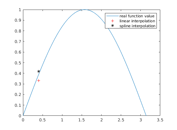
The spline interpolation uses the information about the convexity, we can see that the spline interpolant is concave.
Fitting a polynom of a given degree
The previous two interpolation techniques had one thing in common: the 'estimated' function value over the known points were the measured values. We might give an other condition: the sum of the distances squared should be the smallest possible assuming we use a certain type of function to interpolate. In our case we are going to use polynomial that have a degree at most n.
The outputs of this polyfit command are coefficients of the (at most) two degree polynomial which fits our data best.
coeffs=polyfit(x,y,2)
coeffs =

   -0.4011    1.2614   -0.0027
The problem of finding the most fitting one degree polynomial is called linear regression.
We can estimate our function's value by substituting into the polynomial:
value1=polyval(coeffs, point1)
value1 =

    0.4377
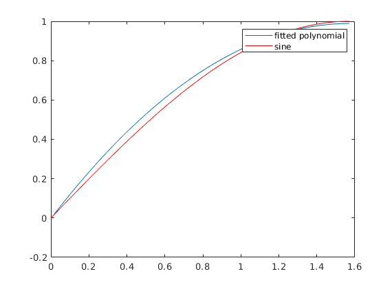
Plotting the polynom and the sine function:
t=linspace(0,pi/2);
plot(t,polyval(coeffs,t), t, sin(t),'r')
legend('fitted polynomial', 'sine')
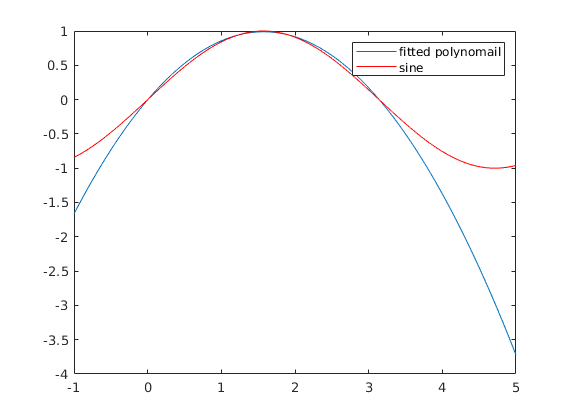
However...
t=linspace(-1,5);
plot(t,polyval(coeffs,t), t, sin(t),'r')
legend('fitted polynomail', 'sine')
Recommended problems
1. Write a function called linEst(v1,v2), which takes two vectors as input. These two vectors are the x and y coordinates of our measured data points. Find the most fitting straight line in least square sense, and plot it with the data points. The output of your function is the steepness of the straight line.
2. Our data point are the following: the x coordinates are (0.5, 1, 1.5, 2, 2.5, 3, 3.5) the y coordinates are (3.27, 6.1, 9.7, 12.9, 15.1, 19.4, 21.3). Write a function called estMate(n), which takes a positive integer as input. The function calculates the best fitting at most n degree polynomial, and plots it and the data points. The function also saves the plot to an jpg file.
3. Write a function called rungeCo(n), which takes a positive integer as input. The function calculates the best fitting at most n-1 degree polynomial for the following problem: we take n equidistant points on the interval [-5,5]. These point are the x coordinates of our data points. The y coordinates are 1/(1+x^2). Plot the f(x)=1/(1+x^2) function and the fitted polynomial for n=5 and n=15.
4. Write a function called interpolals(x,y,x0) which takes two vectors (x and y coordinates of the data points), and a floating point number x0. The output of your function is the estimated function value in x1 using spline interpolation.