In this section, we will study a two-parameter family of distributions that has special importance in probability and statistics.
The beta function, first introduced by Leonhard Euler, is defined as follows:
Show that the beta function is well-defined, that is, for any and , using these steps:
Show that
Show that the beta function can be written in terms of the gamma function as follows:
Show that if and are positive integers, then
Let's generalize this result. First, recall the generalized permutation formula from our study of combinatorial structures: for , , and , we defined
Suppose that , , , and . Show that
Show that
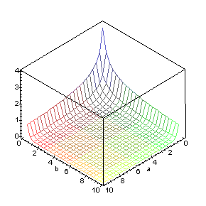
A graph of on the square is shown below.

Show that the function below is a probability density function for every
The distribution with the density in the previous exercise is called the beta distribution with left parameter and right parameter . The beta distribution is useful for modeling random probabilities and proportions, particularly in the context of Bayesian analysis. The distribution has two parameters and yet a rich variety of shapes:
Sketch the graph of the beta probability density function. Note the qualitative differences in the shape of the density for the following parameter ranges:
In the random variable experiment, select the beta distribution. Set the parameters to values in each of the ranges of the previous exercise. In each case, note the shape of the beta density function. Run the simulation 1000 times with an update frequency of 10 and note the apparent convergence of the empirical density function to the true density function.
The special case , is the arcsine distribution (the name will be explained below). Thus, the probability density function of the arcsine distribution is
In some special cases, the beta distribution function and its inverse, the quantile function , can be computed in closed form. In the following exercises, denotes the left parameter and the right parameter, as usual.
Suppose that and . Show that
Suppose that and that . Show that
Suppose that (the arcsine distribution). Show that
In general, there is an interesting relationship between the distribution functions of the beta distribution and the binomial distribution.
Fix . Let denote the binomial distribution function with trial parameter and success parameter , and let denote the beta distribution function with left parameter and right parameter , where . Show that
Hint: Express as an integral of the beta probability density function, and then integrate by parts.
In the quantile applet, select the beta distribution. Vary the parameters and note the shape of the density function and the distribution function. In each of the following cases, find the median, the first and third quartiles, and the interquartile range. Sketch the boxplot.
The moments of the beta distribution are easy to express in terms of the beta function.
Suppose that has the beta distribution with left parameter and right parameter . Show that
Suppose that has the beta distribution with left parameter and right parameter . Show that
In particular, if , so that has the arcsine distribution, then and
In the simulation of the random variable experiment, select the beta distribution. Set the parameters to values in each of the ranges of Exercise 8. In each case, note the size and location of the mean/standard deviation bar. In each case, run the simulation 1000 times with an update frequency of 10. Note the apparent convergence of the sample moments to the distribution moments.
Suppose that has the gamma distribution with shape parameter and scale parameter , that has the gamma distribution with shape parameters and scale parameter , and that and are independent. Show that has the beta distribution with left parameter and right parameter .
Suppose that has the beta distribution with left parameter and right parameter . Show that has the beta distribution with parameters left parameter and right parameter .
Suppose that has the distribution with degrees of freedom in the numerator and degrees of freedom in the denominator. Show that
has the beta distribution with left parameter and right parameter .
Suppose that has the beta distribution with left parameter and right parameter . Show that the distribution is a two-parameter exponential family with natural parameters and , and natural statistics and .
The beta distribution is also the distribution of the order statistics of a random sample from the uniform distribution.
The beta distribution can be easily generalized from the support interval to an arbitrary bounded interval where , using a linear transformation. Thus, suppose that has the standard beta distibution with left parameter and right parameter . Defne
Use the change of variables theorem to show that has probability density function
Most of the results in the previous sections have simple extensions to this generalized beta distribution. In particular, the mean and variance are given in the following exercise.
Use Exercise 16 and basic properties of expected value and variance to show that