---

Lesson 11
Nonlinear Programming

---

I. The Pooling Problem

The blending plant in a refinery is composed of a pool and two mixers as shown in the picture below.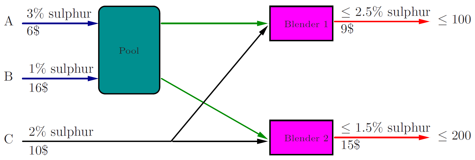


Two types of crude oil A, B whose unitary costs are 6$, 16$ and sulphur percentages are 3%, 1% respectively, enter the pool through two input valves. The output of the pool is then carried to the mixers, together with some crude of type C (unit cost 10%, sulphur percentage 2%) which enters the plant through a third input valve. Mixer 1 must produce petrol containing at most 2.5% sulphur, which will be sold at a unitary price of 9$. Mixer 2 must produce a more refined petrol containing at most 1.5% sulphur, sold at a unitary price of 15$. The maximum market demand for the refined petrol 1 is of 100 units, and of 200 units for refined petrol 2. The goal is to maximize the revenue.

I./1. Problem formulation

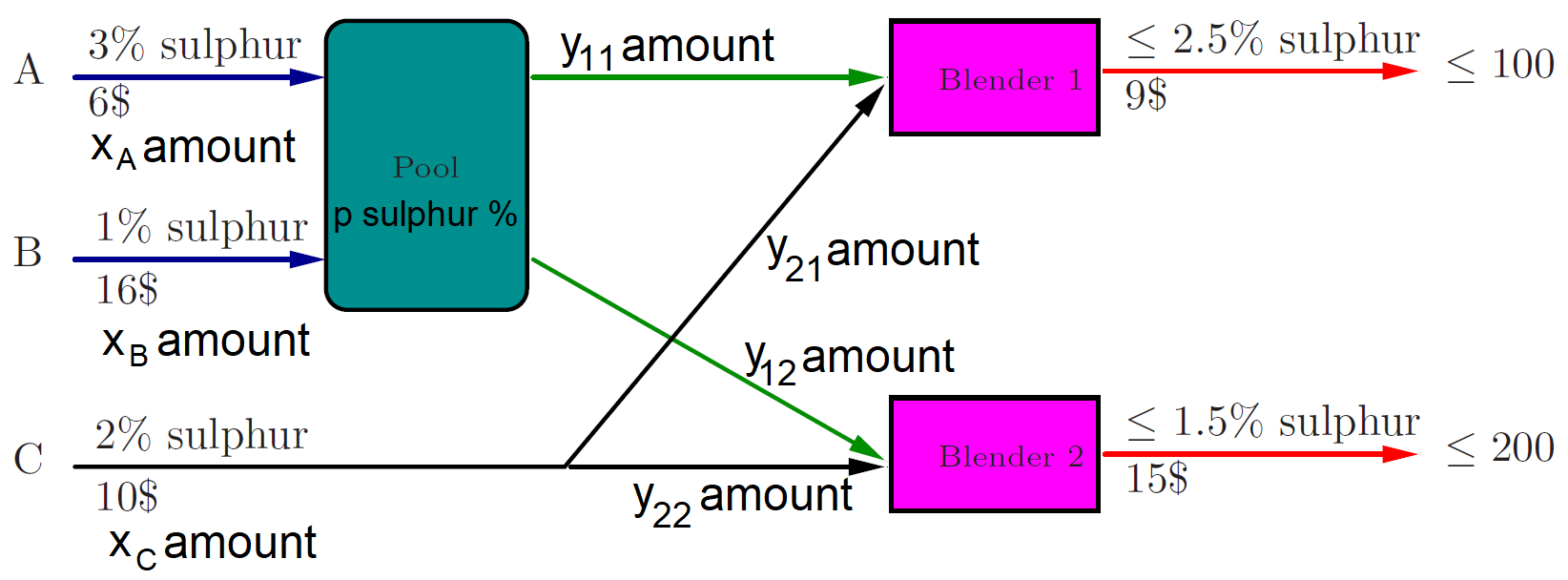
Mass balance constraints: $$\begin{align} x_A + x_B &= y_{11} + y_{12} \\ x_C &= y_{21} + y_{22} \end{align}$$ Market demand constraints: $$\begin{align} y_{11} + y_{21} &\le 100 \\ y_{12} + y_{22} &\le 200 \end{align}$$ Sulphur balance in pool: Instead of explicitly calculating \(p\) with the following equation: $$p = \frac{0.03x_A + 0.01x_B}{x_A+x_B}$$ we don't want to divide by variables, so we'll replace them with \(x_A + x_B = y_{11} + y_{12}\), and multiply my the denominator: $$0.03x_A + 0.01x_B = p(y_{11} + y_{12})$$ Resulting quality demands for petrols 1 and 2: $$\begin{align} py_{11} + 0.02y_{21} &\le 0.025(y_{11}+y_{21}) \\ py_{12} + 0.02y_{22} &\le 0.015(y_{12}+_{y22}) \end{align}$$ Download the Lesson11_Pooling.mos Mosel model from here

I./2. Exercise 1

a) Run the code! It shows an error. What is the issue?
b) Is the problem bilinear?
c) Change \(p\) from an mpvar to a real and fix its value to something you feel is appropriate. Solve the problem! Whose solution has the maximum profit?
d) Change \(p\) back to an mpvar! Import "mmxnlp" as well and solve the problem!

I./3. The Haverly Recursion Algorithm

For any bilinear problem with variables \(p\) and \(y\) multiplied together:

1. Set an error bound \(\varepsilon > 0\).
2. Change \(p\) to a constant and set it to (random) starting value.
3. Solve the problem and obtain solution \(\hat{y}\).
4. Change \(y\) to a constant and set its value to \(y=\hat{y}\). Change \(p\) back to a decision variable.
5. Solve the problem and obtain solution \(\hat{p}\).
6. If \(p\) hasn't changed by more than \(\varepsilon\) since the last iteration, output the solution. Otherwise go to 7.
7. Change \(p\) to a constant and set its value to \(p=\hat{p}\). Go to 3.

The algorithm constantly swaps \(p\) and \(y\) between a constant and a decision variable, and finds the optimum for either one. The program swaps between solving 2 different LPs, with constantly changing parameters. This is implemented into mmxnlp.

Note: If \(p\) or \(y\) hasn't changed at all since the last iteration, then we found the optimal solution.

I./4. Exercise 2

a) Look at the solution! Have we found the optimum?
b) How do we know we didn't run into a local optimum?
c) Is the problem convex?
d) Is the problem concave?
e) In general, how can you decide if an optimization problem is convex?
f) Suggest an algorithm to solve a trilinear problem! (With constraints including \(xyz\), where \(x\), \(y\), and \(z\) are all decision variables.)

II. Separable non-linear problems

Separation Theorem

Let us assume a constraint or the objective function contains the non-linear term \(xy\), where neither \(x\) or \(y\) are binary. Then $$xy = a^2-b^2 \Leftarrow \begin{cases} a = \frac{1}{2}(x+y) \\ b = \frac{1}{2}(x-y)\end{cases}$$ Where the \(f(a)=a^2, f(b)=b^2\) functions can be approximated with a piecewise linear funtion. (Remember, \(b\) could take on negative values as well.)

Note: Linearizing \(\left(\sum_{i=1}^n x_i\right)\left(\sum_{i=1}^n y_i\right)\) works the same way by setting \(a = \frac{1}{2}\left(\sum_{i=1}^n x_i + \sum_{i=1}^n y_i\right)\), and \(b = \frac{1}{2}\left(\sum_{i=1}^n x_i - \sum_{i=1}^n y_i\right)\). There is no need to multiply together term by term!

III. Quadratic production example

Our production planning team has observed that the amount of motor fuel we sell versus we put on inventory is in a tight balance. Whenever we leave the following ellipse in a given period, the next planning period will be very rough: $$(x-30)^2-\frac{3}{2}(x-30)(y-30)+(y-30)^2 \le 350$$ where \(x\) is the amount (in kt) we put on inventory from motor fuel in the given period, and \(y\) is the amount we sell (in kt).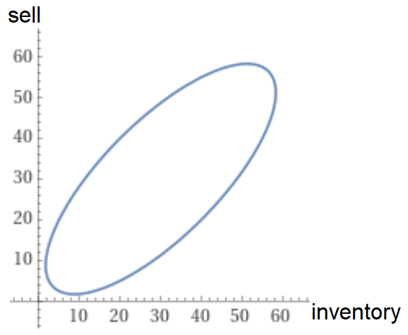
However our sales management team has observed that this period we will need to sell 4 times as much motor fuel than the amount we put on inventory, to keep up with market demand.

How much motor fuel should we produce? How much of it should we sell versus put on inventory?

III./1. Exercise 3

a) Formulate the problem and solve it in XPress using mmxnlp!
b) What (else) could be the objective function?
c) How many decision variables would we need if we used the Separation Theorem to get only squared terms?

IV. Bacteria production example (again)

Download the Lesson4_Bacteria.mos Mosel model from here (again)

IV./1. Exercise 4

a) Import mmxnlp!
b) Change OBJ from linctr to nlctr, and uncomment OBJ!
c) Run the program! Is the constraint OBJ >= goal satisfied? If not, why not?
d) Is the problem convex?