---

Lesson 5
Modelling conditional constraints, abs & sign

---

I. Modelling conditional (if) constraints with LP and IP

We have already seen and used these types of constraints:

Conditional modelling Theorem 1

Let \(a, x \in \mathbb{R}^n, r \in \mathbb{R}, b \in \{0,1\}\), and let \(x,b\) be unknown, and \(a,r\) be known. Then $$\begin{cases} b=0 \Rightarrow a^Tx \le r \\ b=0 \Leftarrow a^Tx < r \\ b=1 \Rightarrow a^Tx \ge r \\ b=1 \Leftarrow a^Tx > r\end{cases} \quad \Longleftrightarrow \quad \begin{cases} a^T x b \ge rb \\ a^T x - r \le bM \end{cases}$$ for any \(M \ge \sup(a^T x - r)\)

We've actually already used this condition in the Backpacks example: $$\begin{align} &\sum_{i \in \text{ ITEMS}} \text{rope}(b)\text{packing}(b,i)\text{weights}(i) \ge \text{rope}(b)\text{ropeMin} \\ &\sum_{i \in \text{ ITEMS}} \text{packing}(b,i)\text{weights}(i) - \text{ropeMin} \le \text{rope}(b)M \end{align}$$

Conditional modelling Theorem 2

Let \(a, x \in \mathbb{Z}^n, r \in \mathbb{Z}, b \in \{0,1\}\), and let \(x,b\) be unknown, and \(a,r\) be known. Then $$\begin{cases} b=0 \Leftrightarrow a^Tx \le r-1 \\ b=1 \Leftrightarrow a^Tx \ge r\end{cases} \quad \Longleftrightarrow \quad \begin{cases} a^T x b \ge rb \\ a^T x - r + 1 \le bM \end{cases}$$ for any \(M \ge \sup(a^T x - r + 1)\)

This is almost the same Theorem, but in the case of integer variables, we can actually split the range of \(a^T x\) into two non-intersecting regions, which we couldn't do in the continuous case, because we can't model strict inequalities like \(a^T x - r < 0\).

Absolute Value modelling Theorem

Let \(x \in \mathbb{R}\), then $$ y=|x| \Longleftrightarrow \begin{cases}y = 2xb-x \\ xb \ge 0 \\ x \le bM\end{cases}$$ for any \(M \ge \sup(x)\); where we introduced the \(b \in \{0,1\}\) binary decision variable.

Sign modelling Theorem

Let \(x \in \mathbb{R}\), then $$\begin{cases} x < 0 \Rightarrow y = -1 \\ x > 0 \Rightarrow y = 1\end{cases} \Longleftarrow \begin{cases}y = 2b-1 \\ xb \ge 0 \\ x \le bM\end{cases}$$ for any \(M \ge \sup(x)\); where we introduced the \(b \in \{0,1\}\) binary decision variable.

Note that all 4 Theorems include instances of \(xb\), which is two variables multiplied together. In order to actually use these Theorems, one should use Lesson 3's Linearization Theorem 1 or 2 to linearize these expressions.

II. Manhattan distance maximization example

Place 5 points on the edges of the \([0,1]^2\) unit-square such that their total Manhattan distance from each other is maximal!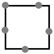

II./1. Excercise 1

a) Create a new Mosel file by opening XPress, navigating to the green + icon, and using New \(\rightarrow\) Mosel file.
b) Create a parameter for the number of points (5), and create the range POINTS from 1 to the number of points!
c) Create a parameter for the number of sides (4), and create the range SIDES from 1 to the number of sides!
d) Declare the following variables:

• x: array on POINTS, decision variable, the x coordinate of each point
• y: array on POINTS, decision variable, the y coordinate of each point
• side: array on (POINTS,SIDES), binary decision variable, 1 if the given point is on the given side
• distances: array on (POINTS,POINTS), decision variable, the distances between points \(i\) and \(j\)

e) Set up the following constraint: All points should land on exactly one side.
f) Set up 4 constraints of this type (this encodes what \(x\) and \(y\) should be if they are on the bottom side of the unit-square): $$\forall p \in \text{POINTS, if } \text{side}_{sp} = 1 \Rightarrow 0 \le x_p \le 1;\ y_p=0$$ g) Linearize the above constraints using one of the Theorems we've learned!
h) Define \(\text{distances}(i,j)\) for all \(i,j \in \{1,\dots,5\}\) to be $$\text{distances}(i,j) := |x_i - x_j| + |y_i - y_j|$$ i) Linearize \(\text{distances}(i,j)\) using the Absolute Value modelling Theorem.
j) Set the objective value to be the sum of all distances calculated.
k) Maximize the objective function and run the program.
l) Optional: Set \((x_1,y_1)=(0,0)\) for a more consistent output.

II./2. Excercise 2

Open another Mosel file! Place 7 points on the faces of the \([0,1]^3\) unit-cube such that their total Manhattan distance from each other is maximal!


Differences:

• Now you will need another array of decision variables for the 3rd coordinate, z.
• Now you will need a 6-long array for the sides instead of 4.
• The Manhattan distance will change to \(\text{distances}(i,j) := |x_i - x_j| + |y_i - y_j| + |z_i - z_j|\)