Lesson 8
Quadratic Programming
I. Portfolio selection with Quadratic Programming
We would like to make a portfolio (= investment strategy). There are 10 shares available that we can invest into, and we would like to determine what proportion of our investment should go into each share. We have a target of 10 USD that we would like to earn.From historical data, we have calculated the covariance between each pair of share, and we've obtained the following covariance matrix:
$$\text{Cov}(X,X) = \begin{bmatrix} 0.1 & 0 & 0 & 0 & 0 & 0 & 0 & 0 & 0 & 0 \\ 0 & 19 & -2 & 4 & 1 & 1 & 1 & 0.5 & 10 & 5 \\ 0 & -2 & 28 & 1 & 2 & 1 & 1 & 0 & -2 & -1 \\ 0 & 4 & 1 & 22 & 0 & 1 & 2 & 0 & 3 & 4 \\ 0 & 1 & 2 & 0 & 4 & -1.5 & -2 & -1 & 1 & 1 \\ 0 & 1 & 1 & 1 & -1.5 & 3.5 & 2 & 0.5 & 1 & 1.5 \\ 0 & 1 & 1 & 2 & -2 & 2 & 5 & 0.5 & 1 & 2.5 \\ 0 & 0.5 & 0 & 0 & -1 & 0.5 & 0.5 & 1 & 0.5 & 0.5 \\ 0 & 10 & -2 & 3 & 1 & 1 & 1 & 0.5 & 25 & 8 \\ 0 & 5 & -1 & 4 & 1 & 1.5 & 2.5 & 0.5 & 8 & 16 \end{bmatrix}$$ This means that for example \(\text{Cov}(X_2,X_3)=-2\), so as one is expected to go up, the other is expected to go down (rapidly).
Additionally, the expected return of each share is known:
$$\mathbb{E}_{\text{return}}(X) = \begin{bmatrix} 5 & 17 & 26 & 12 & 8 & 9 & 7 & 6 & 31 & 21 \end{bmatrix}$$ We are interested in minimizing the total variance of our investment while making sure the total expected return stays above 10 USD. Let us denote the fraction of our money invested into share \(i\) with \(\text{frac}(i)\), then we are minimizing: $$\text{Var}_X(\text{frac}) = \sum_{s \in \text{ SHARES}}\ \sum_{t \in \text{ SHARES}} \text{Cov}(X_s,X_t)\text{frac}(s)\text{frac}(t)$$
I./1. Exercise 1
a) Why is this the total variance? What does the product \(\text{Cov}(X_s,X_t)\text{frac}(s)\text{frac}(t)\) refer to?b) This objective function isn't linear. Look up the definition of the Quadratic Programming model! Does this fit into its definition? Why?
I./2. Exercise 2
Download the Lesson8_Portfolio.mos Mosel model from hereDownload the investment.dat Data file from here
a) Go through the model and understand the constraints!
b) What other method of diversifying our investment can you think of? Is it easier or harder to model that?
c) Why are we investing the maximum amount possible into share 1?
d) Go to lines 49-53! Model the connection between invest(s) and frac(s) using the Theorems learnt in the previous lessons!
e) Why does the total variance grow, even though we're investing into fewer shares overall?
II. The quadratic backpack problem
The class going on a tour. There are 7 types of items we can bring with us (any number of any item), but we have limited carrying capacity (500 kg overall). Each pair of items have a cross-value. This value is high if the items are useful together, and low if they are not so useful together. This cross-value ranges from 0 to 9. For example:High cross-value examples:
can + can opener
pot + lighter
pot + water
pen + paper
flashlight + battery
Low cross-value examples:
water + pen
battery + paper
flashlight + pot
can opener + pen
coca cola + mentos
What items and how many should we bring with us?
II./1. Exercise 3
Download the quadraticBackpackData.dat Data file from herea) Create a new Mosel file!
b) Define a range (1 to 7) for the number of items, and declare maximum weight as 500.
c) Create the arrays weights and crossValues and initialize them from the above Data file.
d) Define variables that'll store how many of each item we'll bring with us! Set them to integer.
e) Import "mmquad" and define the objective function as a qexp type variable!
f) Define a constraint that we cannot bring more than 500 kg of items with us.
g) Define the objective function, which should be the total value of the brought items. (If we are bringing \(a\) of item \(i\) and \(b\) of item \(j\), then we should add \(a\cdot b \cdot \text{crossValue}(i,j)\) to the objective function!)
h) Maximize the objective function!
i) Print out the total cross-value and exactly how many of each item we brought!
j) Import "mmsystem" and measure how long the program runs for!
k) Why does this program take significantly longer to run than the previous one? (There is one key difference!)
III. Eucledean distance maximization example
Place 5 points on the edges of the \([0,1]^2\) unit-square such that their total Euclidean distance from each other is maximal!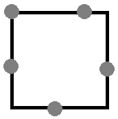
III./1. Excercise 4
a) Create a new Mosel model! If you have already done this in Lesson 5, then you can just copy your model and modify it!b) Create a parameter for the number of points (5), and create the range POINTS from 1 to the number of points!
c) Create a parameter for the number of sides (4), and create the range SIDES from 1 to the number of sides!
d) Declare the following variables:
- x: array on POINTS, decision variable, the x coordinate of each point
- y: array on POINTS, decision variable, the y coordinate of each point
- side: array on (POINTS,SIDES), binary decision variable, 1 if the given point is on the given side
- distances: array on (POINTS,POINTS), decision variable, the distances between points \(i\) and \(j\)
f) Set up 4 constraints of this type (this encodes what \(x\) and \(y\) should be if they are on the bottom side of the unit-square): $$\forall p \in \text{POINTS, if } \text{side}_{sp} = 1 \Rightarrow x_p=0;\ 0 \le y_p \le 1$$ g) Linearize the above constraints using Conditional modelling Theorem 1.
h) Define \(\text{distances}(i,j)\) for all \(i,j \in \{1,\dots,5\}\) to be $$\text{distances}(i,j) := (x_i - x_j)^2 + (y_i - y_j)^2$$ i) Set the objective value to be the sum of all distances calculated.
j) Maximize the objective function and run the program.
k) Optional: Set \((x_1,y_1)=(0,0)\) for a more consistent output.
l) Compare the result to the Manhattan distance example!
III./2. Excercise 5
Open another Mosel file! Place 7 points on the faces of the \([0,1]^3\) unit-cube such that their total Euclidean distance from each other is maximal!
Differences:
- Now you will need another array of decision variables for the 3rd coordinate, z.
- Now you will need a 6-long array for the sides instead of 4.
- The Euclidean distance will change to \(\text{distances}(i,j) := (x_i - x_j)^2 + (y_i - y_j)^2 + (z_i - z_j)^2\)